Introduction to JAX

First order derivative

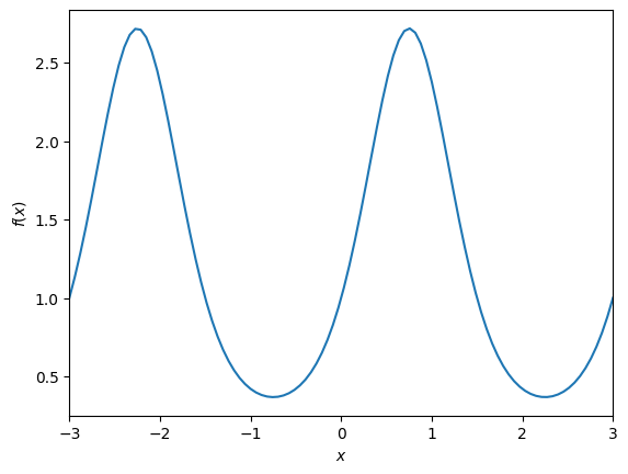
JAX is Python library that allows you, among others, to compute derivatives of functions automatically. Here is a toy example on how to use the jax.grad function. We compute both analytic and automatic differentiation of the following function:

\[f(x)=\exp{(\sin(\frac{2 \pi x}{3}))}\]

From which the derivative is : $\(f^{'}(x) = \frac{2 \pi}{3} cos(\frac{2 \pi x}{3}) \exp(sin(\frac{2 \pi x}{3}))\)$

First we define the function and its derivative and plot \(f\).

import jax
import jax.numpy as jnp

import numpy as np
import matplotlib.pyplot as plt


def func(x):
    arg = jnp.sin(2 * jnp.pi * x / 3)
    return jnp.exp(arg)


def symbolic_grad(x):
    arg = 2 * jnp.pi * x / 3
    return 2 * jnp.pi / 3 * jnp.exp(jnp.sin(arg)) * jnp.cos(arg)


x = jnp.linspace(-3, 3, 100)
plt.plot(x, func(x))
plt.xlabel(r"$x$")
plt.ylabel(r"$f(x)$")
plt.xlim(x.min(), x.max())

(-3.0, 3.0)

Then we define the derivative function with jax.grad and we check that both the hand-derived function and the automatic differentiated function match for a random value of \(x\).

grad_func = jax.grad(func)
print(grad_func(0.5))
np.testing.assert_allclose(grad_func(0.5), symbolic_grad(0.5)) #This tests if the two arguments (arrays) are matching one another within a tolerance.

2.4896522

Now that we are confident with the implementation of the gradient function we can also check the matching of both for multiple values of \(x\). In this regard we plot both functions and compare the plots.

plt.plot(x, jax.vmap(grad_func)(x), label="AD")
plt.plot(x, symbolic_grad(x), "--", label="symbolic")
plt.xlabel(r"$x$")
plt.ylabel(r"$\mathrm{d} f(x) / \mathrm{d} x$")
plt.xlim(x.min(), x.max())
plt.legend()

<matplotlib.legend.Legend at 0x7fe59cbf3140>

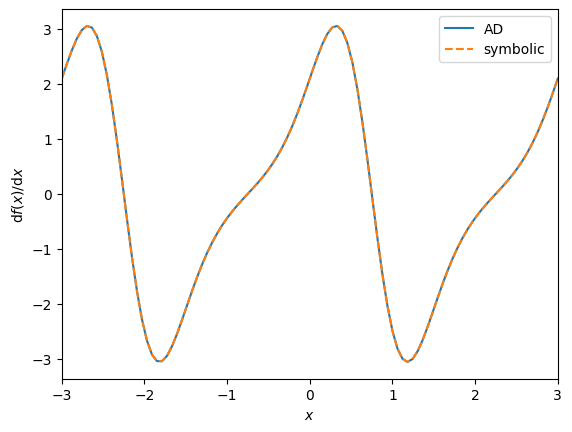
You can see that both functions perfectly match.

Higher order derivatives

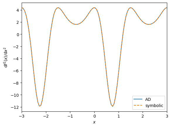
You can obtain higher order derivatives following the same process. In this section we compute the second order derivative of the function defined above : $\(f^{''}(x) = \left(\frac{2 \pi}{3}\right)^{2} \left(cos(\frac{2 \pi x}{3})^{2} \exp(sin(\frac{2 \pi x}{3})) - sin(\frac{2 \pi x}{3}) \exp(sin(\frac{2 \pi x}{3})) \right) \)$

def symbolic_grad_grad(x):
    arg = 2 * jnp.pi * x / 3
    u = jnp.exp(jnp.sin(arg))
    u_prime = 2 * jnp.pi / 3 * jnp.cos(arg) * jnp.exp(jnp.sin(arg))
    v = jnp.cos(arg)
    v_prime = -2 * jnp.pi / 3 * jnp.sin(arg)
    return 2 * jnp.pi / 3 * (u_prime * v + u * v_prime)

Same as before we use jax.grad to obtain the derivative of the derivative.

grad_grad_func = jax.grad(jax.grad(func))
print(grad_grad_func(0.5))
np.testing.assert_allclose(grad_grad_func(0.5), symbolic_grad_grad(0.5)) #This tests if the two arguments (arrays) are matching one another within a tolerance.

-6.4243035

We plot the symbolic function and the one obtained with JAX and compare both on a plot

plt.plot(x, jax.vmap(grad_grad_func)(x), label="AD")
plt.plot(x, symbolic_grad_grad(x), "--", label="symbolic")
plt.xlabel(r"$x$")
plt.ylabel(r"$\mathrm{d} f^{2}(x) / \mathrm{d} x^{2}$")
plt.xlim(x.min(), x.max())
plt.legend()

<matplotlib.legend.Legend at 0x7fe59c76c860>

One application : gradient based optimization

So far we have been presenting how to automatically compute the gradient of a function with JAX. In this section we present a toy example of gradient based optimization.
The optimization method is a gradient descent method : you start at \(x_0\) and evaluate gradient at this point.
We use a fixed learning rate to update the \(x_k\) position at every step according to : \(x_{k+1} = x_k - \alpha _k f^{'}(x_k)\).
The gradient \(f^{'}(x_k)\) of the objective function is obtained through automatic differentiation with JAX. The value of the learning rate \(\alpha _k\) is arbitrary but should be \(\in ]0,1]\)

import jax
import jax.numpy as jnp

import numpy as np
import matplotlib.pyplot as plt

The objective function we are trying to minimize is a quadratic function.

def f_ref(x):
    f = x**2 + 3*x - 5
    return f

The gradient function is defined with jax.grad

grad_function = jax.grad(f_ref)

We compute a very simple gradient descent method where you update the position of the minimum depending on the value of the gradient at the current \(x_k\).

def optimizer(x0,f,grad_function,tol):

    gradient_f = grad_function(x0)
    x_k = x0
    alpha_zero = 0.07
    iter = 0

    alpha_k = alpha_zero

    while abs(gradient_f) > tol :
        
        x_k = x_k - alpha_k * gradient_f
        gradient_f = grad_function(x_k)
        iter+=1

    return(x_k,f(x_k),iter)
    

Let’s now run the optimizer for which we provide the gradient function defined above and print the \(x_{min}\) found.

x_min,f_min,iter = optimizer(-2.5,f_ref,grad_function,1e-3)
print(x_min,f_min,iter)

-1.5004565 -7.25 51

As you can see this method is extremely inefficient especially with fixed rates. The closer you get to the solution, the closer the gradient goes to zero and the smaller the step you take is.
There is no reason to use gradient descent in optimization but it is not in the scope of this class to present more efficient methods.